Oscilloscope

Introduction

Antares' oscilloscope component can capture signal values at various points in a circuit and display how these signals change over time as graphical signal curves.

Unlike similar tool which don’t treat component propagation delays, Antares simulates components with individual propagation delays, and the oscilloscope is capable of displaying the resulting timing differences, which can help you trouble-shooting subtle timing problems in your circuit designs.

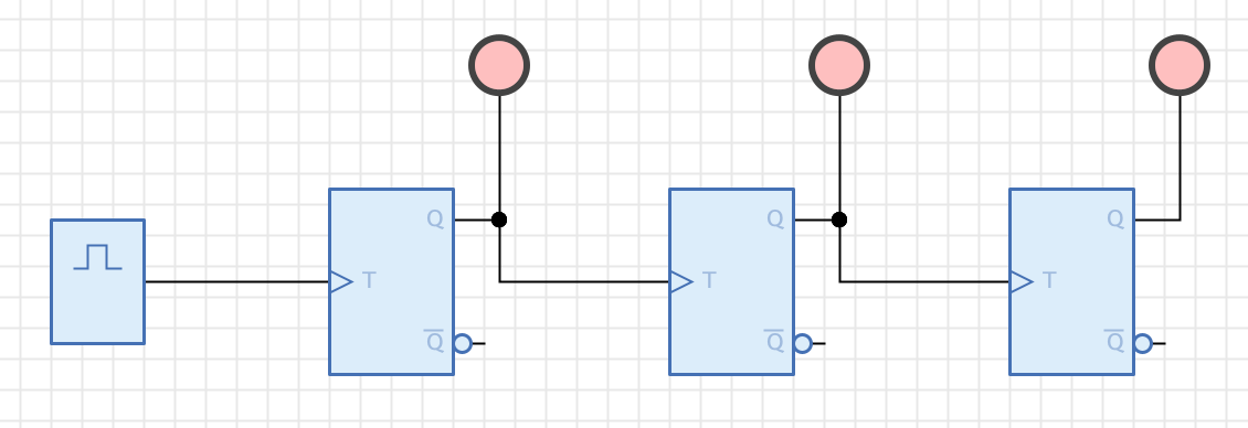
Let’s explain how the oscilloscope is used by going through an example circuit. Assume you have a counter circuit like below. Since such a counter circuit can also be viewed as a frequency divider, we want to set up an oscilloscope that nicely shows how frequencies are divided during simulation.

Adding the Oscilloscope

Selecting View  Oscilloscope creates a new, empty oscilloscope component and adds it to your circuit.

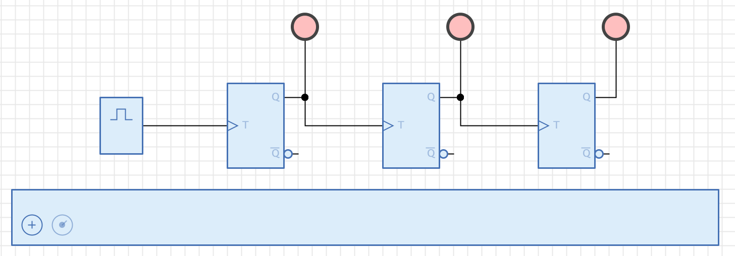
Technically, the oscilloscope is just a circuit component like any other. After you added it to the circuit, the circuit can be saved, and all changes you’ve made to the oscilloscope will be saved within the circuit.

However, once created and added to the circuit, the oscilloscope can be hidden by deselecting View  Oscilloscope again. This sets the "visible" property of the oscilloscope to "false", a change that can also be saved.

When the oscilloscope is initially added to a circuit, it is positioned just below the circuit. You can select it and move it to another position, which is then stored when the circuit is saved.

To get rid of an oscilloscope, just select and delete it. The next time you select View  Oscilloscope, a newly initialized oscilloscope will be created.

Since oscilloscopes come with a certain overhead, tend to avoid adding them to low-level library circuits you plan to use multiple times in project circuits. You can use an oscilloscope while designing low-level circuits, but consider removing the oscilloscope from library circuits once their design is stable.

Adding Oscilloscope Rows and Probes

An oscilloscope consists of up to 8 rows, each of which has a signal probe and a signal curve. To add a new row, click on the + button at the bottom of the oscilloscope. Each click adds a new row initially named by its index.

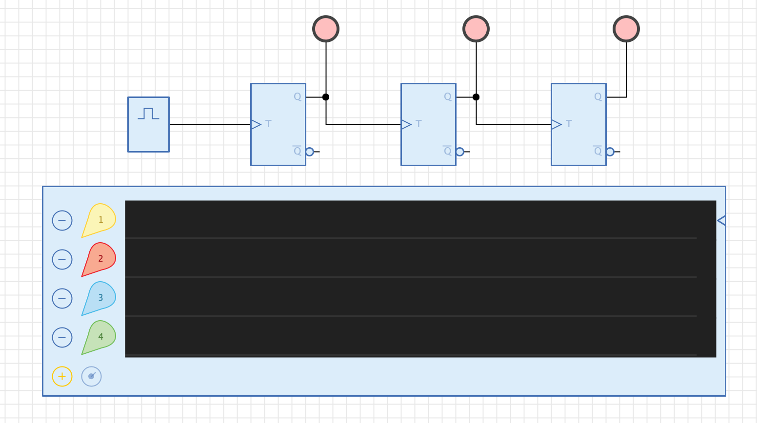
The bubble-shaped icon at the start of a row represents the signal probe. Click it with the mouse and drag it into the circuit.

Think of this like the probe of a particular row has been taken off its slot in the oscilloscope and moved into the circuit where it should capture signals. An empty slot in the oscilloscope is drawn only as outline, while the effective probe is always drawn as a filled icon.

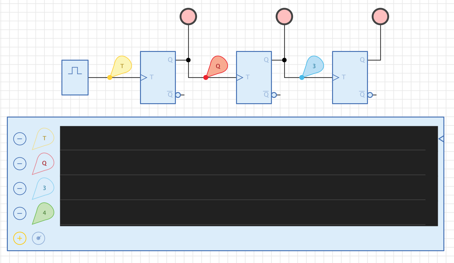
Probes only capture signals if they are connected to a wire, which is indicated by a small circle at the tip of the probe. You can place a probe anywhere else in the circuit, but then it won’t capture signals.

Also notice how the name of a probe changes if you drop it on a circuit’s wire. Antares uses a strategy to automatically determine the name of a probe depending on where it has been dropped. This strategy tries to use names from components and input/output ports that participate in the net to which the probe has been added. If there is no such name, or the evaluated name is not unique, Antares uses a generic, unique name.

You can change the automatically assigned probe name by selecting the probe and entering the new name in the properties view. Antares will ensure that all probe names are unique.

You can also rotate a selected probe in the circuit using Cmd R.

To remove a probe from the circuit, just select and delete it. Antares will then move it back to its slot in the oscilloscope.

Removing entire rows can be achieved by pressing the - button at the start of a row. If the row’s probe has previously been dragged into the circuit, it will be deleted as well.

Simulation in "Clocked" Mode

The oscilloscope supports different timing modes. You can choose the mode by selecting the oscilloscope and changing the value of is property "Mode" in the properties panel. Newly created oscilloscopes have mode "Clocked" by default. Clocked mode is also designated in the oscilloscope component by a small triangle at the right side of the first row.

In clocked mode, the captured signal curves don’t represent the real simulation time, but an artificial "oscilloscope time" that leads to evenly alternating signal curves, because signals are captures only when the signal at the first (clocked) row changes. This can be convenient because large time differences between signal changes (such as microsecond clocks and nanosecond gate propagation delays) are "normalized" to the artificial, evenly spaced "oscilloscope time". The drawback of clocked mode is that propagation delay subtleties are not shown.

Start the simulation and observe how the signal curve of each row evolves while the circuit is driven by the clock component.

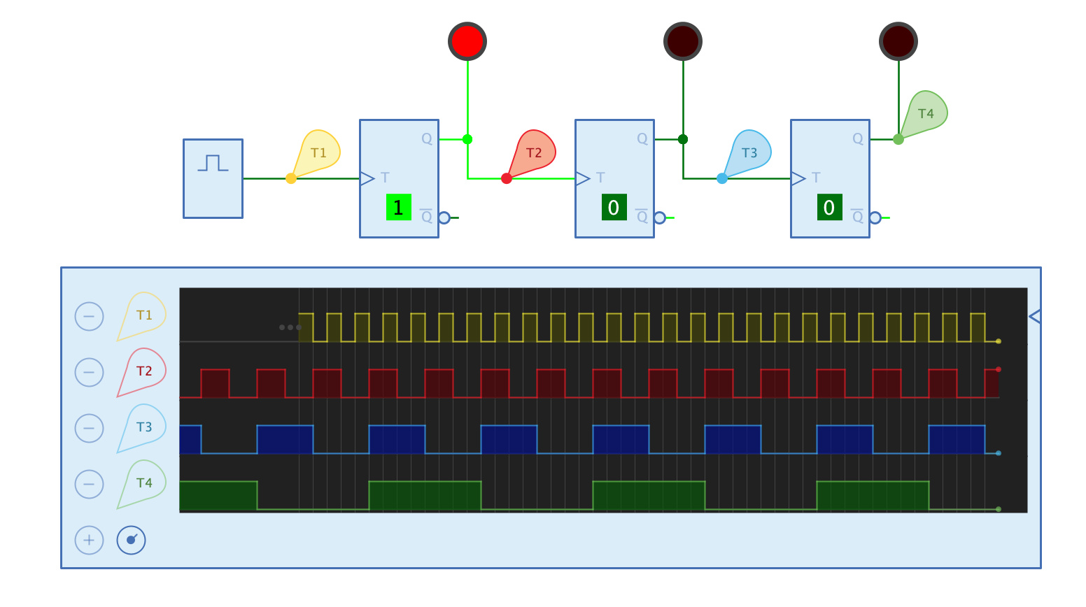
The oscilloscope has a "Scaling" property that scales the signal curve when being drawn on the screen. Set the default scaling value in the oscilloscope’s property, or change it during simulation by hovering over the knob button at the bottom of the oscilloscope and adjusting the scale by turning the popup knob. Press/hold the left mouse button while turning the know around its center.

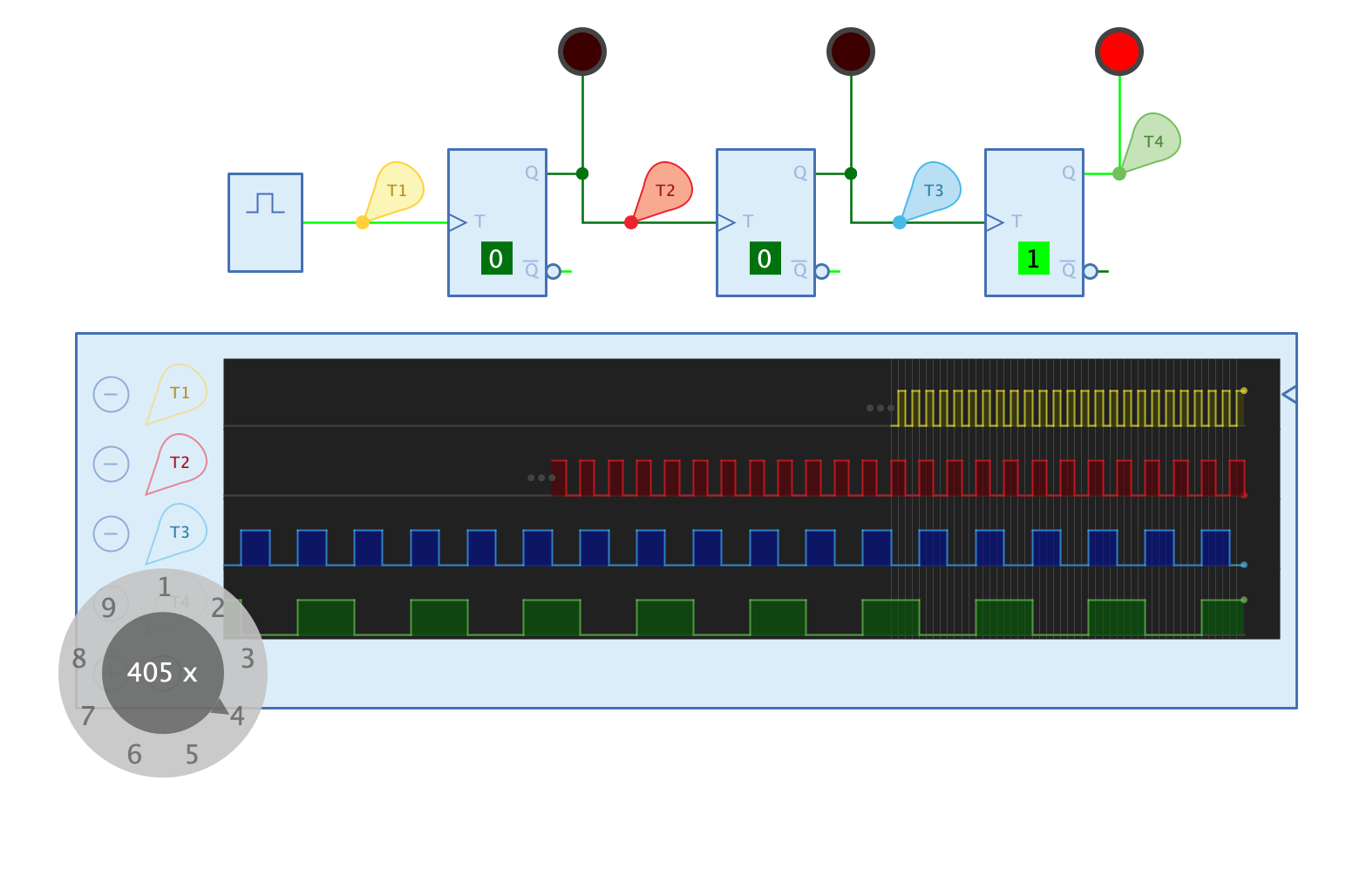
Note also the three gray dots in the first and second rows. These indicate that there are no more data values available for the given point in time. Antares only stores a certain number of captured signals; if this number is reached, older values are deleted. You can configure this number in the user preferences (see below).

Simulation in "Real-Time" Mode

In "Real-Time" oscilloscope mode, the oscilloscope uses the real simulation time when capturing signal changes in the circuit. Therefore, real propagation delays of circuit components become transparent in signal curves.

Let’s demonstrate this by equipping the "Pulse Generator" circuit from Antares' standard library with an oscilloscope in order to analyse the circuit’s timing in detail. Remember that this circuit creates a short pulse at its output "O" for every rising edge at its input "I".

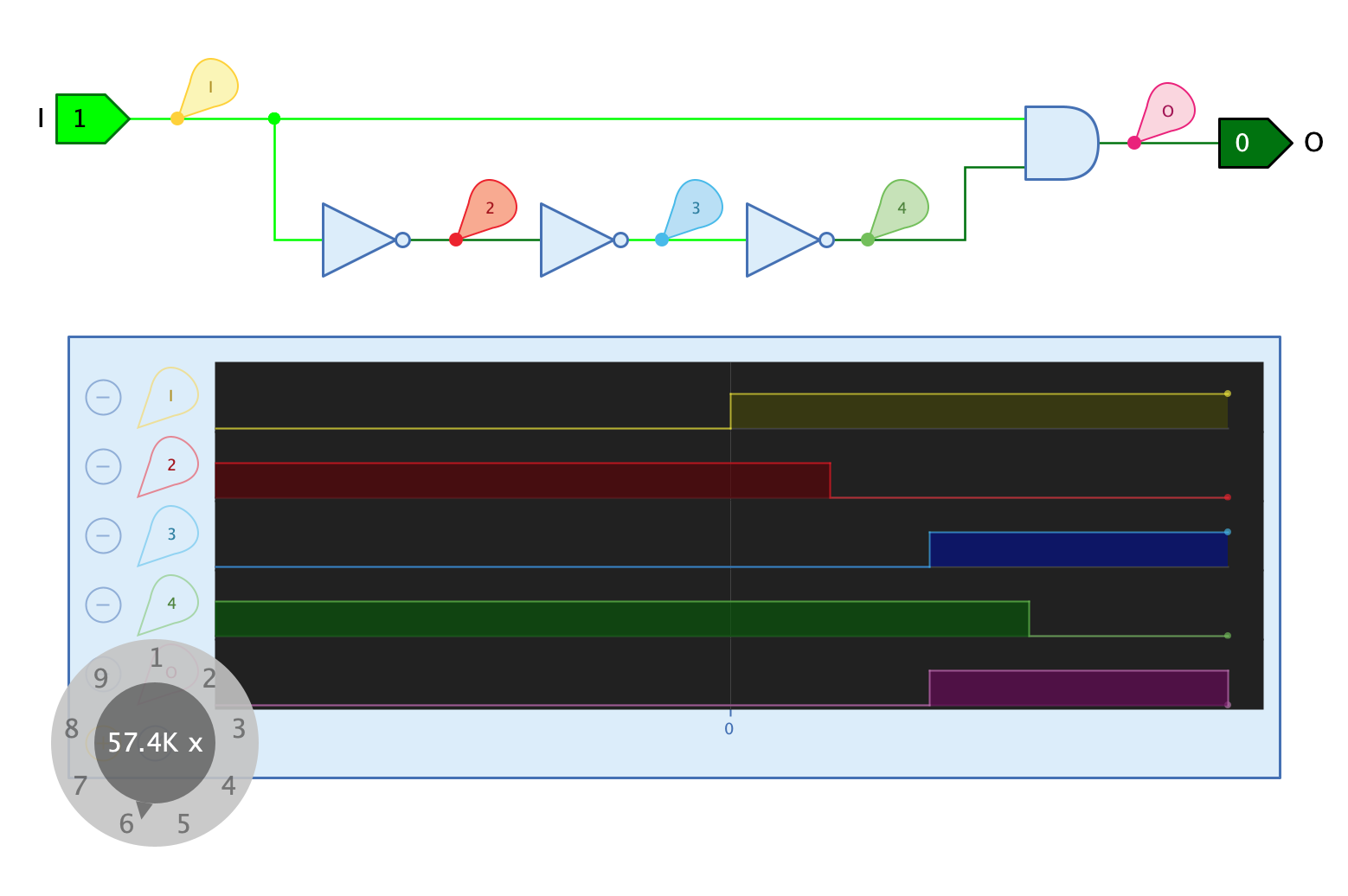
Note how the propagation delay of the AND gate ultimately determines the length of the generated output pulse, and how it is driven by the accumulated NOT gate propagation delays.

In order to make the timing subtleties nicely visible, the oscilloscope’s scale had to be scaled up to around 57'000.

User Preferences

Antares' user preferences allows you to configure certain aspects of oscilloscope behaviour and looks.

Max. number of signal values

The maximum number of signals stored in each oscilloscope row. If this number is reached, older captured signal values are deleted.

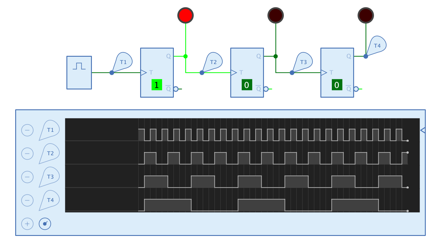
Individual probe colors

Determines whether oscilloscope signal curves and probes have an individual color (default). If you deselect this property, all signal curves and probes have the same color, whose value depends on the current theme.

Fill signal curve

Determines whether signal curves are filled or not.