Simulation

Simulation Tools

The simulation of Antares is controlled by the simulation tools in the toolbar. The most important actions can also be performed using the keyboard or menus.

With this button (Ctrl+R) the simulation can be started and stopped.

Pauses or resumes the simulation (Space). The button turns orange if simulation is paused.

Activates the single step mode of the simulation.

If single step mode should pause simulation with every new signal being generated, make sure to select menu option Simulation  Soft Breakpoints. Otherwise, only "hard breakpoints" from the "Break Component" are used.

With the slider the simulation speed can be controlled. The simulation speed is divided into three categories whose names are displayed as a tooltip when you move the mouse over the slider. The further to the left the slider is, the slower the simulation is executed and the more support information is displayed during simulation.

The speed categories have the following names:

Use

This category is mainly used to use a circuit without displaying more details about how it works. For example, if you have finished designing a microprocessor circuit and are running machine programs in it that you want to see the results of, you will move the controller all the way to the right to make the simulation run as fast as possible.

Observe

This category displays support information that can be useful during the development of a circuit without running the simulation much slower.

Explore

This category displays all available support information, if enabled in the settings. In particular, the signal flow animations (if enabled) used in this category slow down the simulation so much that you will use this category mainly for demonstrations or training.

The following table shows which support information is used in which area.

Information	Explore	Observe	Use
Active components
Execution Animation	()	()	()
scenarios	()	()	()
Colored wires
Mnemonics
ROM/RAM-memory contents
Display Execution Delay	()
Signal flow animation

() Only in single step mode

Signal colors

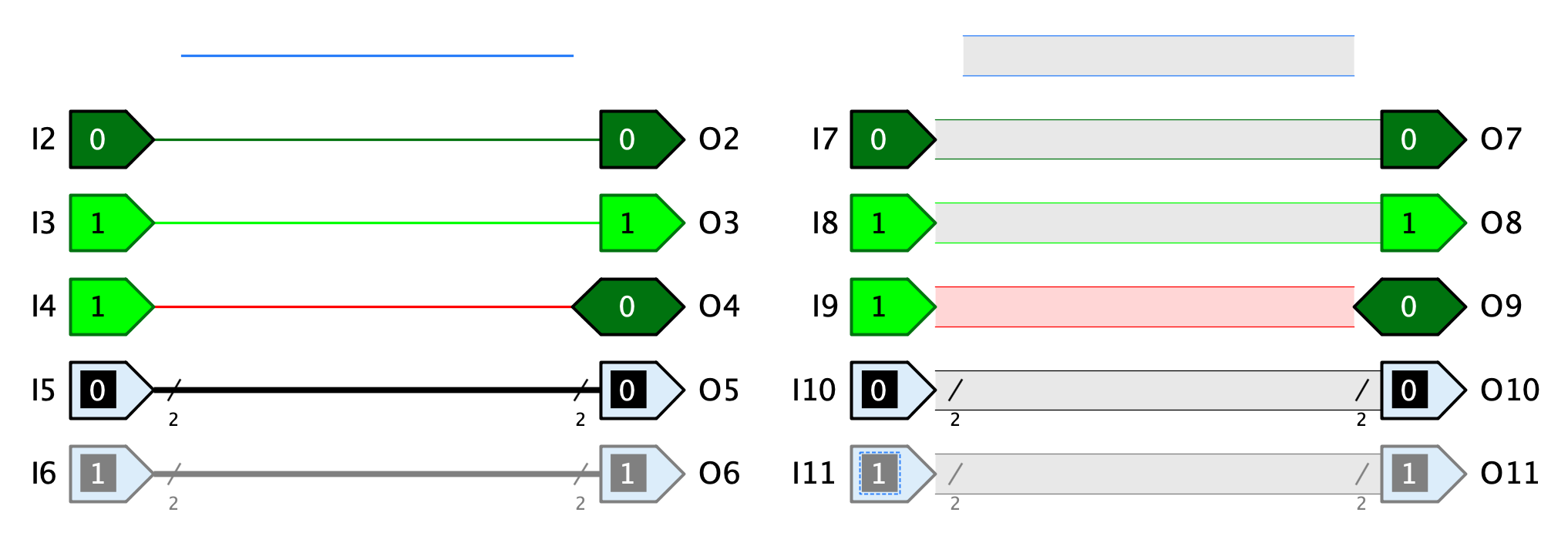
Antares uses different colors during simulation to represent the different values of signals or the states of wires and pins. The following circuit illustrates the colors used, where the wires on the left have the wire style "Line" and the wires on the right have the wire style "Block".

• Blue The wire carries a signal with value "undefined". This occurs if no component is sending a signal to the wire, either because it is not connected to a component or because a connected tri-state buffer is sending an undefined signal.

• Dark green: The wire carries a 1-bit signal with the value 0.

• Light green: The wire carries a 1-bit signal with the value 1.

• Red: The wire carries a signal in which at least one bit has the value "Error". This can occur if several components transmit different signals on the same wire.

• Black: The wire carries a signal with several bits which all have the value 0.

• Gray: The wire carries a signal with several bits, at least one of which has the value 1.

Colors are defined in Antares by "Themes". The themes currently contained in Antares all use the above colors. However, it is not excluded that in the future more themes will be added (or users may define their own themes) that use other colors.

Simulation depth

One of the most important design goals of Antares is to enable the user to explore all the components of a circuit in order to understand its operation as deeply and thoroughly as possible. For this reason, the basic library contains rather few built-in components. Instead, standard components like flip-flops or registers are available as modelled subcircuits in the standard library, which the user can open and observe during circuit design and simulation.

The disadvantage of this approach is that large circuits consist of many basic components if all subcircuits are expanded for simulation until only basic components are used. For example, the microcomputer in the example project "Microcomputer (Tanenbaum)" contains (when fully expanded) over 2'000 elementary logic gates and over 5'000 wires.

The simulation of such large circuits takes a lot of time. Now Antares offers the possibility to define a Execution script for a subcircuit, which contains the logic of the subcircuit and is executed during simulation instead of the inner circuit.

With the menu Simulation  Deep Simulation you can choose whether Antares applies the execution scripts of subcircuits or not. "Deep Simulation" means that the execution scripts are not applied and Antares simulates the full depth of the circuit. The opposite is called "Flat Simulation": Subcircuits are simulated only as deep as the depth of the circuit until a subcircuit contains an execution script.

A flat simulation has one important limitation: If you open a subcircuit containing an execution script during a flat simulation, Antares can display the contents of the subcircuit, but it can’t tell you anything about the state of the components and wires of that subcircuit.

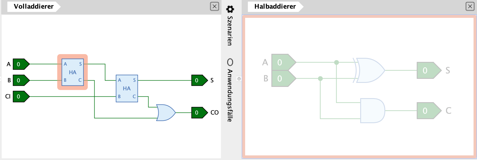
Antares therefore represents such a subcircuit in a "disguised" state. In the picture above, one of the half adders has been opened in a separate view. Antares shows the opened half adder with a grey overlay. If the subcircuit would contain another subcircuit, you could also open it or dive into it, but it would also be shown in a disguised state.

Simulation algorithm

Antares' algorithm for simulating circuits is usually not something you need to understand in detail to use Antares. Therefore, this section only explains the basics.

Signal values

The simulation of Antares uses signals with four possible values 0, 1, "Undefined" (high impedance)" and "Error".

Other simulations use other signals such as "0/1 (rising edge)" and "1/0 (falling edge)". So far, Antares has not shown any need for such extended models.

Propagation delay

The simulation uses the propagation delay defined for each component and each wire. This is the time (in nanoseconds) a component needs to process a changed input signal and generate a corresponding signal at one or more outputs.

The simulation algorithm is event-based. Whenever a component detects a change in an input value, a new entry in an event queue is created in the simulation engine, which is intended to be executed after the propagation delay of the component has expired. After this time has elapsed, the simulator prompts the component to recalculate the value of its outputs. For this calculation, the component uses the signals that exist at its inputs at this time.

Pure net components (wires, splitter, combiner, subcircuit ports) have a propagation delay of zero.

Switch-on behaviour

Antares does not yet contain a mechanism by which the switch-on behaviour can be influenced by the circuits and components. When starting simulation, each component is requested to recalculate its outputs. The propagation delay is also taken into account. If at the time of calculation no signal from other components has arrived at the inputs, it is up to the component to decide how to deal with this at the start. Most components then initially set the inputs to the value 0, which results in an unconnected AND gate having the output value 0 at startup and an unconnected NOT gate having the output value 1.

This behavior must be considered when designing sequential circuits. Without further action, the way the simulation algorithm works and the power-on behavior of Antares will cause an SR latch with NOR gates to go into an illegal state at power-on, or will oscillate indefinitely between the two states.

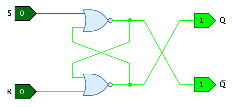
Real latches do not show this behaviour, because slight differences in the propagation delay of the individual gates cause the circuit to settle into a stable and correct state when switched on.

In Antares there are three approaches to achieve the same behavior in simulation as in real circuits.

• Different propagation delays: In the example above, both NOR gates have the same propagation delay, e.g. 10 ns. If different propagation delays are defined for the two gates (e.g. 8 ns for the upper gate and 11 ns for the lower gate), the circuit will settle into a stable, correct state at startup. The latches and flip-flops of Antares' standard library are built according to this approach.

• Noise: With the menu option Simulation  Noise  Random Noise the simulator can be instructed to slightly change the propagation delays of the components by a random value. With this option, the above SR latch takes a correct state at the start of simulation (possibly after a short settling phase), even if both gates have configured the same run-time.

• Power-On Reset: Use a "Power-On Reset" component (introduced with 1.1.0) to bring the circuit into a defined state when the simulation gets started.

Behavior with undefined input values

Certain components like tri-state buffers or bi-directional inputs/outputs can produce undefined (floating) values. The same happens with input ports left unconnected: their signal is assumed to be undefined. On the other hand, logic gates require defined inputs to work properly.

Using the system preference "Undefined Gate Input Behaviour", you can define how Antares behaves during simulation regarding undefined input values. The following options are available.

• Read as 0: An undefined input signal is treated as a 0. This is equivalent to a real logic gate with an integrated pull-down resistors at its inputs.

• Read as 1: An undefined input signal is treated as a 1. This is equivalent to a real logic gate with an integrated pull-up resistors at its inputs.

• Read as random value: An undefined input signal is treated as a random value. If you choose this option, you have to make sure that all input ports are connected, and all tri-state output ports connected to the same input port are coordinated such that a stable signal is always produced, unless your circuits explicitly contains pull resistors that cover these cases.

Bus contention and signal conflicts

While Antares prevents you from connecting more than one output-only port to the same wire, it is often useful to connect various input/output ports to the same wire. It is then up to the circuit logic to avoid that these ports assert different signals to this wire at the same time. If the circuit fails to achieve this, a signal conflict occurs. This often happens due to a timing problem in the circuit, and the signal propagation algorithm of Antares tries to help you to detect and fix these problems.

Whenever an output port asserts a signal to a wire, Antares checks if this signal is in conflict with the signal asserted by any other output port to the same net. The term "net" refers to the combination of all wires that are reachable by this output port, including those behind splitters and combiners, and those that are connected to input ports within subcircuits.

If Antares detects a signal conflict, the signal will not be asserted to the wire. Instead, the behaviour in this situation depends on the value of the following system preferences and settings.

• Preference "Allowed net contention duration": This preference defines how long Antares ignores bus contention situations before issuing a warning or error.

• Menu Simulation  On signal conflict: Defines whether Antares ignores bus contention issues, or whether it issues a warning or an error. The issued warnings or errors are collected in the "Issues" tab of Antares' main window.

• Menu Simulation  Pause on issue: Determines whether the simulation should be paused when an issue occurs. This allows you to analyse the current state of the simulated circuit and to identify the cause of the issue.

If you hover the mouse over a wire in red error state, Antares displays a tooltip containing detailed information about the signal conflict.

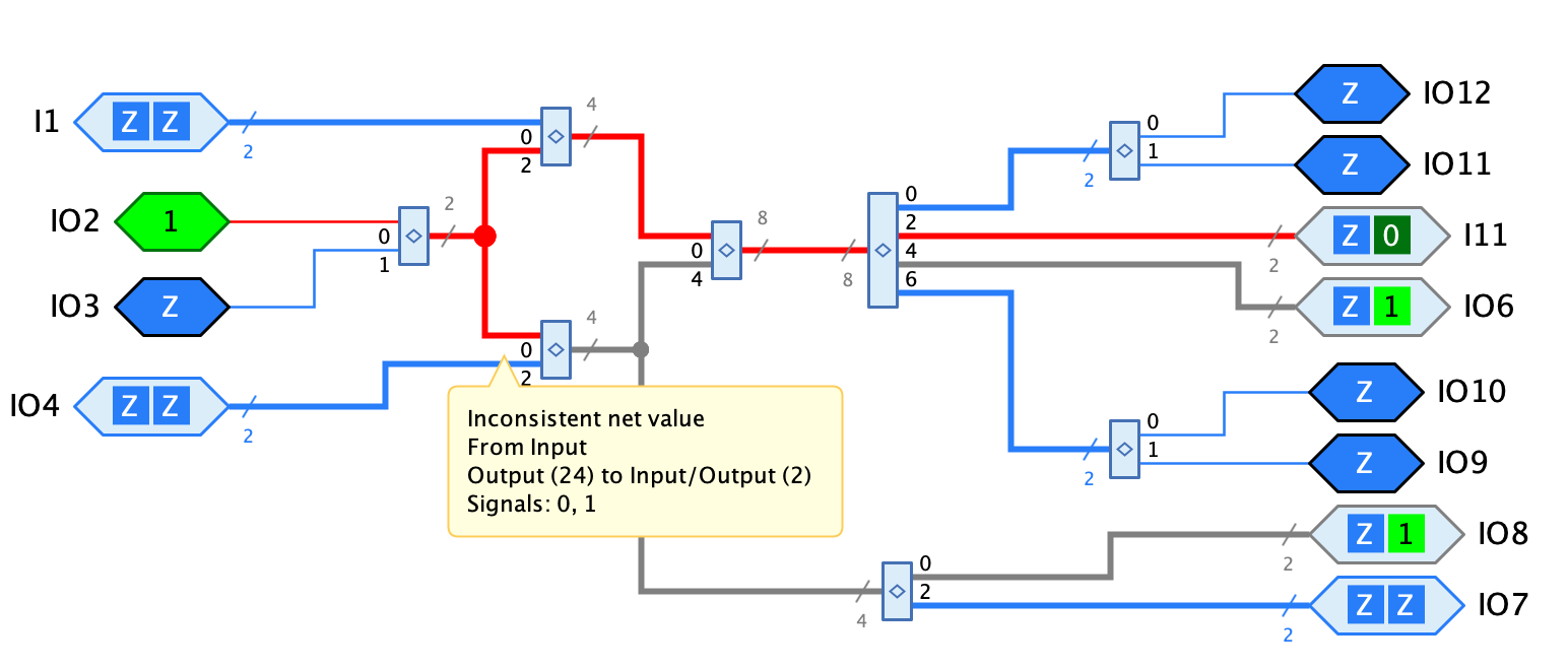
Note that the IDs referenced in the tooltip’s origin and source designations (e.g. 2 in "to Input/Output (2)") reference model ID’s of components. You see these model ID’s in Antares' property panel when selecting a component in the edit mode.

Wire Logic

Starting with release 1.0, Antares supports two different types of "Wire Logic", which determine how the simulation behaves when two different signals are asserted to the same wire.

• Conflict: This is the default value: Different values asserted to the same wire are regared as conflict. See the preceding section for a description of how Antares reacts to conflicts during simulation.

• Wired OR: In this mode, conflicting signals are OR-ed together, allowing you to build circuits based on "Wired OR" behaviour. Every component in the circuit is regarded to be an open-collector device with an internal pull resistor. See Wikipedia’s "Open Collector" article for more detail, or the "Wired OR" article in the German Wikipedia.

You can choose your preferred wire logic in a circuit’s properties. When starting a simulation run, Antares uses the wire logic of the main circuit, even if subcircuits might have a different wire logic property value.